The typical approach is executing several runs of the
EA and plot the
average performance over time (average performance of best-of-run-individual NOT population average).
A good rule of thumb is performing a minimum of 30 runs (of course 50-100 runs is better).
The average performance is better than the best-value-achieved-in-a-set-of-runs but variance should also be taken into account.
You can see two nice examples from
Randy Olson's website:
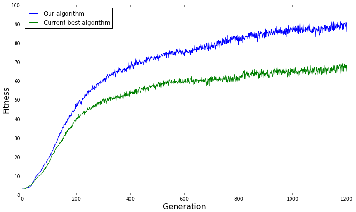 The average fitness of both algorithms over several replicates. From this graph, we would conclude that our algorithm performs better than the current best algorithm on average.
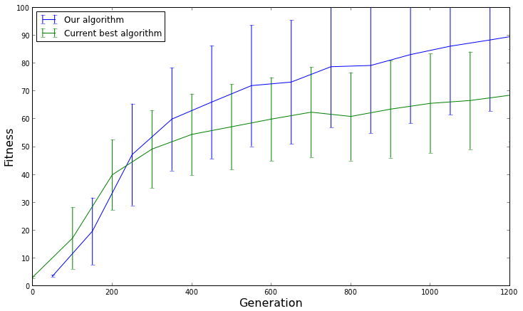 The average fitness with a 95% confidence interval for each algorithm. This graph shows us that our algorithm does not actually perform better than the current best algorithm, and only appeared to perform better on average due to chance.
The basic breakdown of how to calculate a confidence interval for a population mean is as follows:
- Identify the sample mean $\bar{x}$. While $\bar{x}$ differs from $\mu$, population mean, they are still calculated the same way: $$\bar x = \sum {x_{i} \over n}$$
- Identify the (corrected) sample standard deviation $s$: $$s = \sqrt{\frac{\sum_{i=1}^{n}{(x_i - \bar{x})^2}} {n-1}}$$
$s$ is an estimation of the population standard deviation $\sigma$.
- Calculate the critical value, $t^*$, of the Student-t distribution. This value is dependent on the confidence level, $C$, and the number of observations, $n$.
The critical value is found from the t-distribution table (most statistical textbooks list it). In this table $t^*$ is written as $$t^*(\alpha, r)$$ where $r = n-1$ is the degrees of freedom (found by subtracting one from the number of observations) and $\alpha = {1-C \over 2}$ is the significance level.
A better way to a fully precise critical $t^*$ value is the statistical function implemented in spreadsheets (e.g. T.INV.2T function) / scientific computing environments (e.g. SciPy stats.t.ppf), language libraries (e.g. C++ and boost::math::students_t).
- Plug the found values into the appropriate equation:
$$\left({\bar x} - t^{*}{\frac {s} {\sqrt n}}, {\bar x} + t^{*}{\frac {s} {\sqrt n}}\right)$$
- The final step is to interpret the answer. Since the found answer is an interval with an upper and lower bound it's appropriate to state that, based on the given data, the true mean of the population is between the lower bound and upper bound with the chosen confidence level.
The more the confidence intervals of two algorithms overlap, the more likely the algorithms are to perform the same (or we haven't sampled enough to discriminate between the two). If the 95% confidence intervals don't overlap, then the algorithm with the highest average performance performs significantly better.
In EA, the source distribution is essentially never normal and what said so far formally applies only to a normal distribution!
Indeed it still tells many things. The following table summarizes the performance of the t-intervals under four situations:
| Normal curve | Not Normal curve |
|---|
| Small sample size (n<30) | Good | Poor |
| Larger sample size (n≥30) | Good | Fair |
For more accurate answers,
non-parametric statistics are the way to go (see
An Introduction to Statistics for EC Experimental Analysis by Mark Wineberg and Steffen Christensen for further details).
(First revision posted on Computer Science - Stackexchange)